14. Manipulating geographies

Warm up

Go to https://native-land.ca/. This is a crowd-sourced / community-build atlas of indigenous communities’ land before colonization, focused on the Americas and Oceania. Find the place you live now, or where you grew up, or somewhere else familiar to you, and explore it on the map. Are there any names that you recognize as the names of towns, states, rivers, or anything else? Were you familiar with these groups already? Can you think of any other examples of geographic boundaries that are contested, unjust, or could be up for debate?

library(dplyr)
library(ggplot2)
library(sf) 

These are just a few quick notes on how and why you might adjust your geographies. You’ll work through these examples in a practice notebook.

Cartographic boundaries

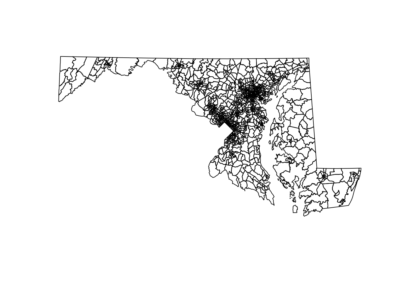
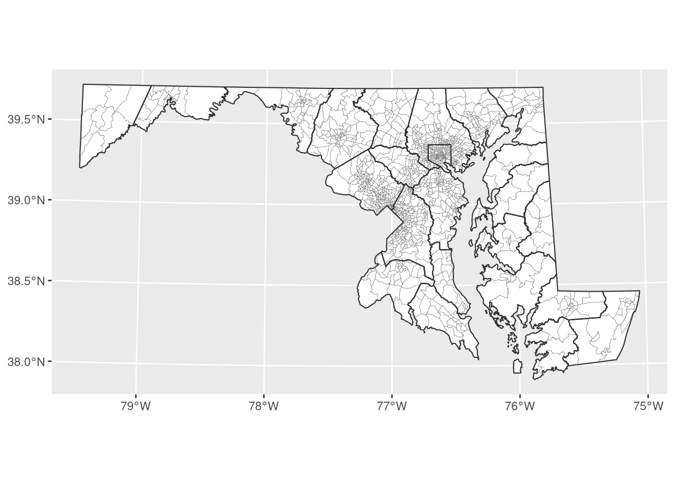
So far we’ve used the Census Bureau’s cartographic boundaries, which are designed for mapping more than for spatial analysis. That’s the cb = TRUE in our previous tigris calls. Now get tracts with this set to false. How are the shapes different? Which has more tracts?

all_tracts <- tigris::tracts(state = "24", cb = TRUE, progress_bar = FALSE) |>
  select(geoid = GEOID, county = NAMELSADCO) |>
  st_transform(2248)

tracts_no_cb <- tigris::tracts(state = "24", cb = FALSE, progress_bar = FALSE) |>
  select(geoid = GEOID) |>
  st_transform(2248)
  
plot(all_tracts$geometry)

plot(tracts_no_cb$geometry)

Combining geometries

Going back to the CB version, we’ll make a map of tracts with county boundaries. With shapefiles from the Census Bureau, we can expect the boundaries to be accurate, but if you’re using data that you’re less confident in, you should know how to aggregate your geometries. (For example, if I map data based on neighborhood boundaries I got from a small town’s city hall with no GIS staff, I’m going to expect there could be some gaps between neighborhoods or boundaries that don’t line up exactly with the official town borders or more high-resolution files from the Census.)

counties <- all_tracts |>
  group_by(county) |>  # add another line here to combine geometries by county
  summarise()

ggplot() +
  geom_sf(data = all_tracts, linewidth = 0.1, color = "gray40", fill = "white") +
  geom_sf(data = counties, fill = NA, linewidth = 0.4, color = "gray20") 

Simplification

Sometimes when you have a lot of shapes, especially very small ones, you’ll want to simplify them. This can make them easier to tell apart in a map, faster to plot (although geom_sf is much faster than when they first added it), and smaller in file size. Imagine a map of counties for the whole US: you don’t need to see all the precise contours of every county. This becomes especially important if you do web mapping. There are different algorithms for how to simplify shapes, but essentially they all remove nodes along the path of a shape.

sf::st_simplify takes a tolerance in meters that signals how far from their original paths the simplified shapes are allowed to go. For small tolerances, you can’t really tell any information has been removed. You’ll experiment with Dorchester County, which has only a few tracts but several small islands.

all_tracts |>
  filter(county == "Baltimore County") |>
  select(geometry) |>
  st_simplify(dTolerance = 50) |>
  plot()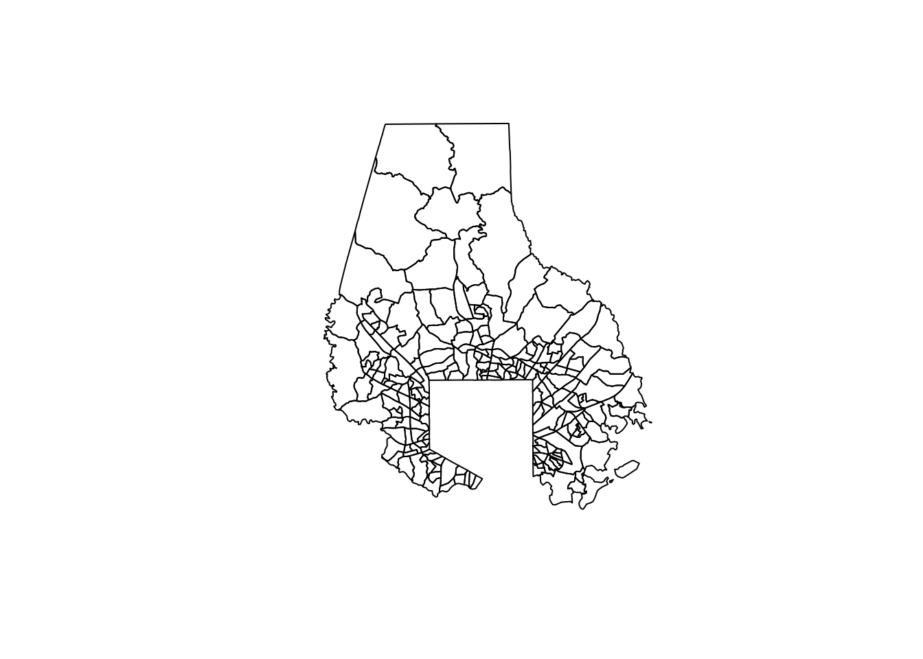

mapshaper is a javascript-based tool to do a lot of geometry manipulation on the command line or in a browser, but there’s an R package that wraps around it. It’s got better simplification algorithms that are less prone to gaps. Instead of a tolerance, you give a percentage of how many nodes to keep—the default is only 5%. Crank the value down until it falls apart.

all_tracts |>
  filter(county == "Baltimore County") |>
  rmapshaper::ms_simplify(keep_shapes = TRUE, keep = 0.8) |>
  select(geometry) |>
  plot()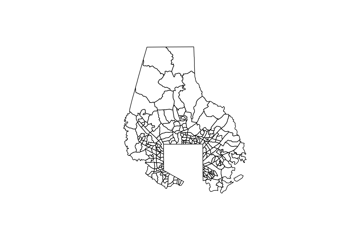

It’s less important here with these smaller data frames, but with larger, more complex data, data in a web app, or data being passed between servers, you’ll want to pay attention to file sizes and memory.

object.size(all_tracts)

2233672 bytes

object.size(all_tracts |> rmapshaper::ms_simplify(keep = 0.2))

1418624 bytes