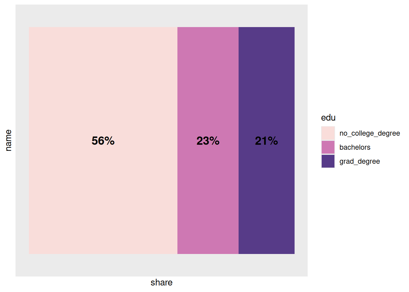
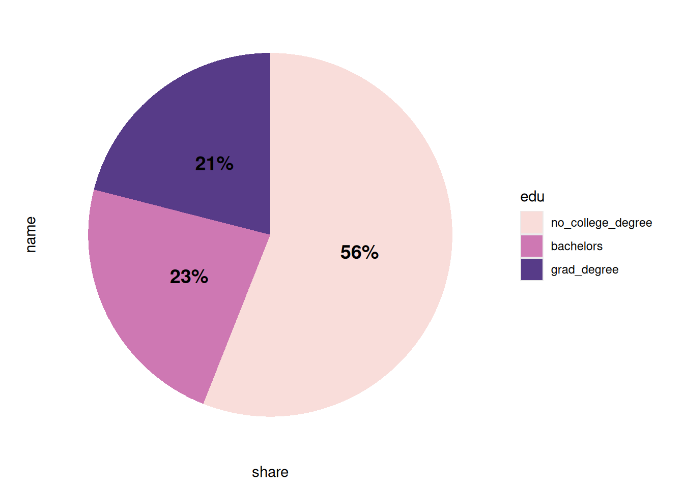
So far when we’ve shown parts of a whole it’s just been stacked bar charts. The elephant in the room is the dreaded pie chart. My general rule is to only use a pie chart for 2 or 3 groups, and only if they’re noticeably different sizes. They should only be used to show mutually exclusive groups within some larger whole (e.g. share of population under/over age 65), and where you don’t need to compare between multiple situations (e.g. only population in Baltimore city but don’t need to compare the city to the county). It’s probably been a few years since I published a pie chart because there’s usually a better option (I really like waffle charts or stacked bars).
As far as ggplot is concerned, a pie chart is a stacked bar chart with radial coordinates and no breaks:
Here are 2 ways of calculating counts and shares, with dummy data set up to mimic two of your datasets:
The first one has 40 observations, where each has a location A or B and a type 1, 2, or 3. If you want to calculate the count of observations of each location-type pair, first count the rows grouped by both location and type, then calculate the share as small group count divided by large group total.
# set a seed for the random number generator so samples are the same each timeset.seed(21)dummy1 <- tibble::tibble(location =rep(c("A", "B"), each =20),type =sample(c("type 1", "type 2", "type 3"), size =40, replace =TRUE))head(dummy1)
location
type
A
type 3
A
type 1
A
type 3
A
type 1
A
type 2
A
type 3
# can do group_by |> summarise, or just count but then add groups back in# I prefer the first method but both get same result:# either thisdummy1 |> dplyr::group_by(location, type) |> dplyr::summarise(n = dplyr::n())
location
type
n
A
type 1
4
A
type 2
9
A
type 3
7
B
type 1
9
B
type 2
7
B
type 3
4
# or thatdummy1 |> dplyr::count(location, type) |> dplyr::group_by(location)
location
type
n
A
type 1
4
A
type 2
9
A
type 3
7
B
type 1
9
B
type 2
7
B
type 3
4
# important part is you need to end up with data grouped by locationdummy1 |> dplyr::group_by(location, type) |> dplyr::summarise(n = dplyr::n()) |> dplyr::mutate(share = n /sum(n))
location
type
n
share
A
type 1
4
0.20
A
type 2
9
0.45
A
type 3
7
0.35
B
type 1
9
0.45
B
type 2
7
0.35
B
type 3
4
0.20
It’s trickier when you have groups that aren’t mutually exclusive, because you can’t just sum observations to get the total number of observations. Instead, you’ll need some way of getting totals beforehand. I do this often enough that I have a function in a work package that extracts groups’ totals based on a label, then calculates shares with those as the denominators. You’re welcome to use that if any of your data is in a format that works for that (it’s how I calculated most of the percentages in our acs dataset with the denominators that are still included there).
In this case, you have a set of observations that each may or may not have one of several traits, marked by TRUE/FALSE. Observations might have more than one trait.
If you don’t need to calculate shares within groups, you can just use the total number of observations as your denominator. Having values as a logical data type means you can just sum them to get the count of TRUEs:
true_false <-c(TRUE, TRUE, FALSE)sum(true_false)
[1] 2
# convert yes/no characters to logical data typeyes_no <-c("yes", "yes", "no")yes_no =="yes"
[1] TRUE TRUE FALSE
sum(yes_no =="yes")
[1] 2
n_obs <-nrow(dummy2)# reshape to long format so you can sum across each traitdummy2_long <- dummy2 |># make trait a factor to keep order tidyr::pivot_longer(-location,names_to ="trait",names_ptypes =list(trait =factor()) )head(dummy2_long)
Note that there are 40 rows in the data, but the total of the column n is 59, because some observations have more than one trait. Dividing by the original number of observations gives the right percentages.
If you need this by group, make a data frame of totals by group before reshaping (I did this wrong the first time around) then join it back to calculate shares:
group_totals <- dummy2 |> dplyr::count(location, name ="group_total")# get counts by both location and traitdummy2_long |> dplyr::group_by(location, trait) |> dplyr::summarise(n =sum(value)) |> dplyr::left_join(group_totals, by ="location") |> dplyr::mutate(share = n / group_total)
location
trait
n
group_total
share
A
is_trait_1
5
13
0.3846154
A
is_trait_2
8
13
0.6153846
A
is_trait_3
4
13
0.3076923
B
is_trait_1
5
16
0.3125000
B
is_trait_2
8
16
0.5000000
B
is_trait_3
9
16
0.5625000
C
is_trait_1
8
11
0.7272727
C
is_trait_2
7
11
0.6363636
C
is_trait_3
5
11
0.4545455
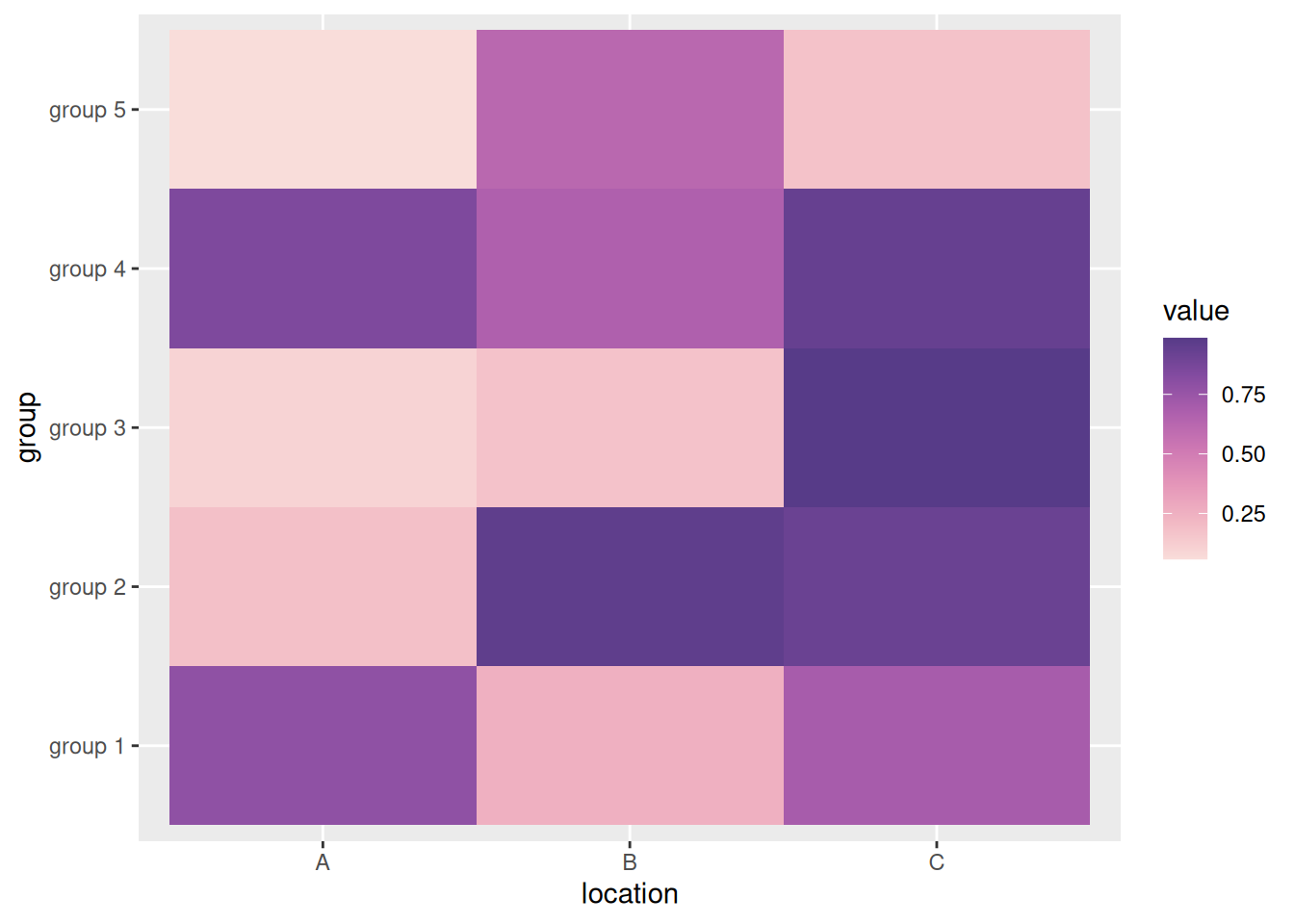
Heatmaps
Since people are interested in heatmaps, here’s an example: