Think back to the first principles we talked about with mapping data onto visual encodings (reading lengths of bar charts, reading darkness of color). With spatial data, we have many of the same principles, but we’re confined by location. We can’t just, say, flip our axes to make them easier to read, or change the aspect ratio to fit in a tight space on a page. We also can’t just arbitrarily change the size of things we’re drawing—for example, in a US state map, we can’t just make Texas less huge.
That said, there are a lot of decisions we do make about how we encode data to space or manipulate it, and these can change the nature of what we know about our data. That makes it important to think really hard about those decisions, and situate those decisions in the purpose of your visualization, your audience, the scope of your work, domain knowledge, etc etc. Often there are no perfectly right answers.
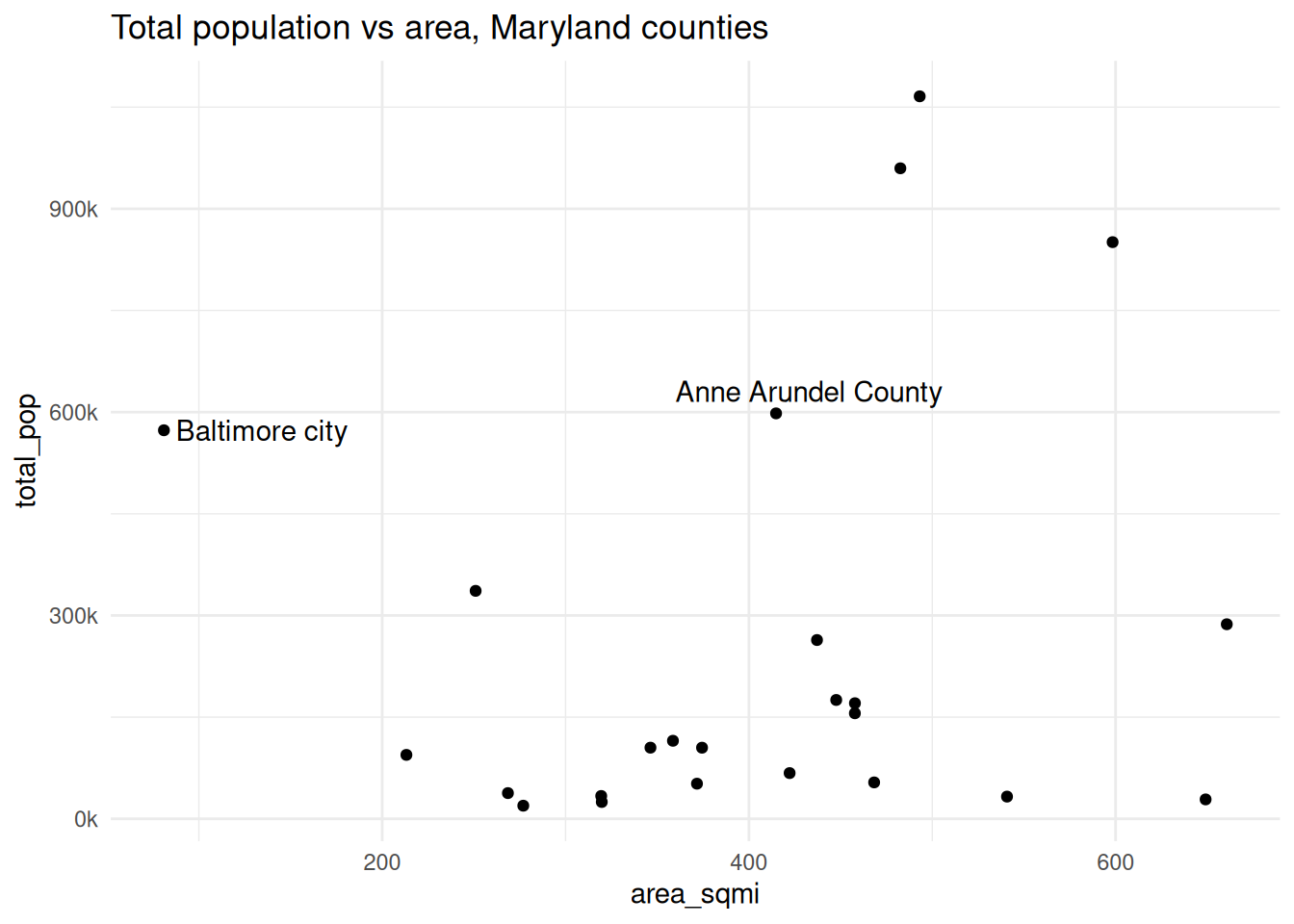
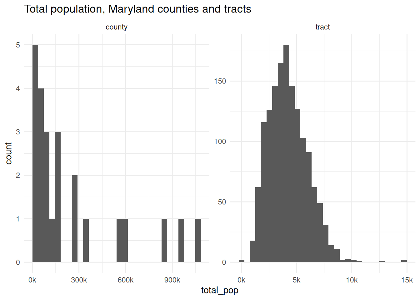
When we looked at Hans Rosling’s bubble plots, the size (area) of points showed the population of each country. That makes sense perceptually—your brain is going to see things of different sizes, pick up on that difference, and think it means something. But in spatial data, it might not; different sizes might actually interfere with our ability to understand what the visual is meant to show. That is, the area of a location might have something to do with the data, but oftentimes it doesn’t (sometimes if anything it shows the opposite—some of the largest US states have among the smallest populations, same goes for Maryland counties). Census tracts are designed to have similar populations, but counties are arbitrary political boundaries.
For example, Baltimore city and Anne Arundel County have similar populations (573k vs 598k), but in the city we’re packed into about 1/5 the area of Anne Arundel County.
Code
library(sf)library(ggplot2)library(patchwork)# justviz::tracts_sf is only baltimore & neighboring countiesall_tracts_sf <- tigris::tracts(state ="24",cb =TRUE,progress_bar =FALSE) |> dplyr::select(geoid = GEOID, county = NAMELSADCO)counties_sf <- all_tracts_sf |> dplyr::group_by(county) |> dplyr::summarise()qual_pal <- rcartocolor::carto_pal(name ="Vivid")theme_set(theme_minimal())
One major issue that comes up in mapping is the modifiable areal unit problem:
The MAUP occurs when statistical results or visual patterns embedded in maps differ according to changes in the scale or zoning of the partitioning scheme used to aggregate spatial data (Openshaw, 1984). The problem commonly occurs when data on individual objects, such as people, are disseminated in data sets in aggregated form, such that the actual spatial distribution of the original individual objects is unobtainable….
One consequence of the MAUP is that spatial patterns that may be observed in a map using one partitioning scheme may not be visible using another partitioning scheme where the scale or zoning differs.
Sometimes the units you use for analysis are ones you can decide on, but sometimes you don’t have a choice (e.g. data would be most useful at the tract level but is only available by town; in a survey you ask for people’s ZIP code because you know they probably don’t know their tract number).
Similar to this is the ecological fallacy, where you assume that patterns or phenomena that you see in aggregate are true for individuals or individual areas within that population.
MAUP and ecological fallacy
When we break a geography into areas that are too large, we lose the patterns that occur within them. If we break into areas that are too small, we might no longer be able to do the analysis we want, or we might be looking at something so closely that patterns aren’t able to develop. For example, counting trees across an entire city won’t tell you anything about tree density in people’s neighborhoods if most of those trees are within one large park; counting trees per parcel in that same city won’t be that useful if you only expect one or two trees at most in front of any house, and if residents get the same benefits of having a tree in front of their neighbor’s house as they do their own.
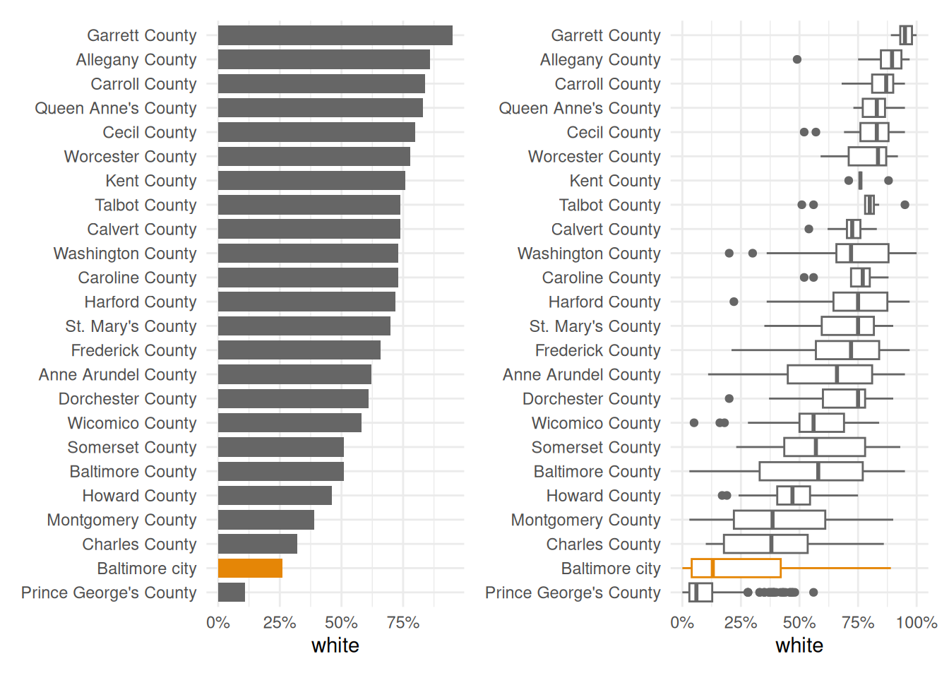
For example, Baltimore city is 26 percent white. That’s the lowest share of all the counties in the state except Prince George’s. But that population is very concentrated within the city.
Even though a much lower share of Baltimore city overall is white than some of the smaller or less diverse counties like Garrett and Carroll, the city is so segregated that we have neighborhoods that do in fact rival those counties’ averages. We lose that fact when we only look at averages or aggregates, but it’s a major pattern underlying much of how the city and region work (hot take: that’s by design).
Choropleths
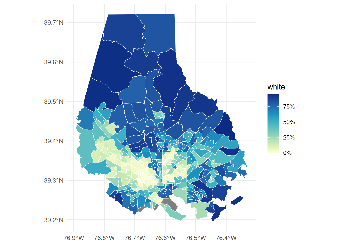
The way I map data is most often a choropleth, where areas are shaded according to a numeric value. There are a lot of considerations, and this is where a lot of those limitations rear their ugly heads, such as having the reader’s understanding of a distribution be distorted by the geographic size of one area. When I weigh the pros & cons of making a choropleth versus a nonspatial chart, I like being able to pair the choropleth with something that gives more exact and specific values, such as a bar chart with city or neighborhood averages.
With choropleths (as with many chart types), you want to be careful about what type of numbers you’re comparing—it should almost always be something standardized into rates, percentages, or other values you’d describe as “x per y units”. With tracts, since they’re of standardized sizes, using counts wouldn’t be as big a deal as with other geographies, but if we showed populations in this way, we’d just be displaying population density. What you’re reading is a value presumably spread over an area, which is why Rankin (2025) refers to choropleths as maps of values (e.g. homeownership rate) per land area. Some types of values that are appropriate for choropleths:
Rankin, W. (2025). Radical cartography: Visual argument in the age of data. Viking.
percentage of population ages 65+
median household income
percentage of households without a car
polling places per 1,000 registered voters
GDP per capita
In most cases, a choropleth would not be appropriate for count of people ages 65+ or total GDP, etc.
With ggplot, simply give your geom_sf shapes color based on some numeric attribute, and you’ve got a choropleth. Here’s another view of the bar and box plots of the white population that makes clear that 1) neither the city nor the county is as uniform as an average would make them seem, and 2) there is very much a spatial pattern that makes a map appropriate.
People have different takes on this, but I find it easier to read, describe, and refer to values in a choropleth when the values are broken into bins and assigned to discrete colors, rather than left continuous and assigned to a continuous gradient. This requires trading away a good deal of precision. We’ll experiment with this in this week’s lab.
Rasters
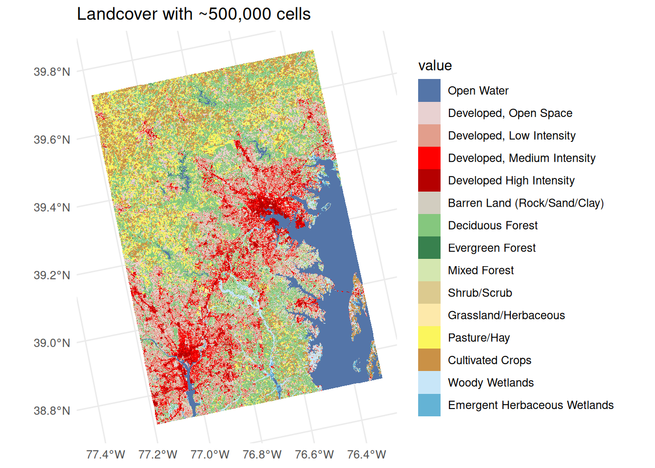
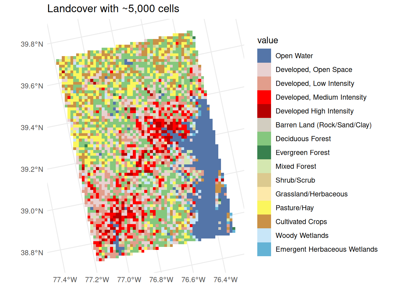
With raster data, we’re also representing data across an area, but in this case the shapes and their areas are fixed. Even when we work with small grid cells of land or water that become single pixels of data, we’re still abstracting and summarizing what happens in that cell. The pixel where my house is in the city is most likely categorized as developed land because that’s the majority of the area. The ecological fallacy would have you believe that’s the entirety of that cell, and you’d miss the lush gardens my neighbors and I have.
Rasterizing data, or converting areal data to gridded or celled data is a way to deal with the MAUP, and we’ll practice that as a technique in a few weeks. But it’s also a bit of a technical solution that might not make sense to people when you’re talking about people-based data. We’re much more accustomed to talking about the values of something for our neighborhood or an area with manmade boundaries than for the 30 meter by 30 meter square that we can’t see and that could change from one data collection process to the next. So in general, we’ll stick to using rasters for data about land, water, and other natural phenomena.
Code
land <- justviz::load_land_cover()ggplot() + tidyterra::geom_spatraster(data = land, maxcell =5e5) +labs(title ="Landcover with ~500,000 cells")
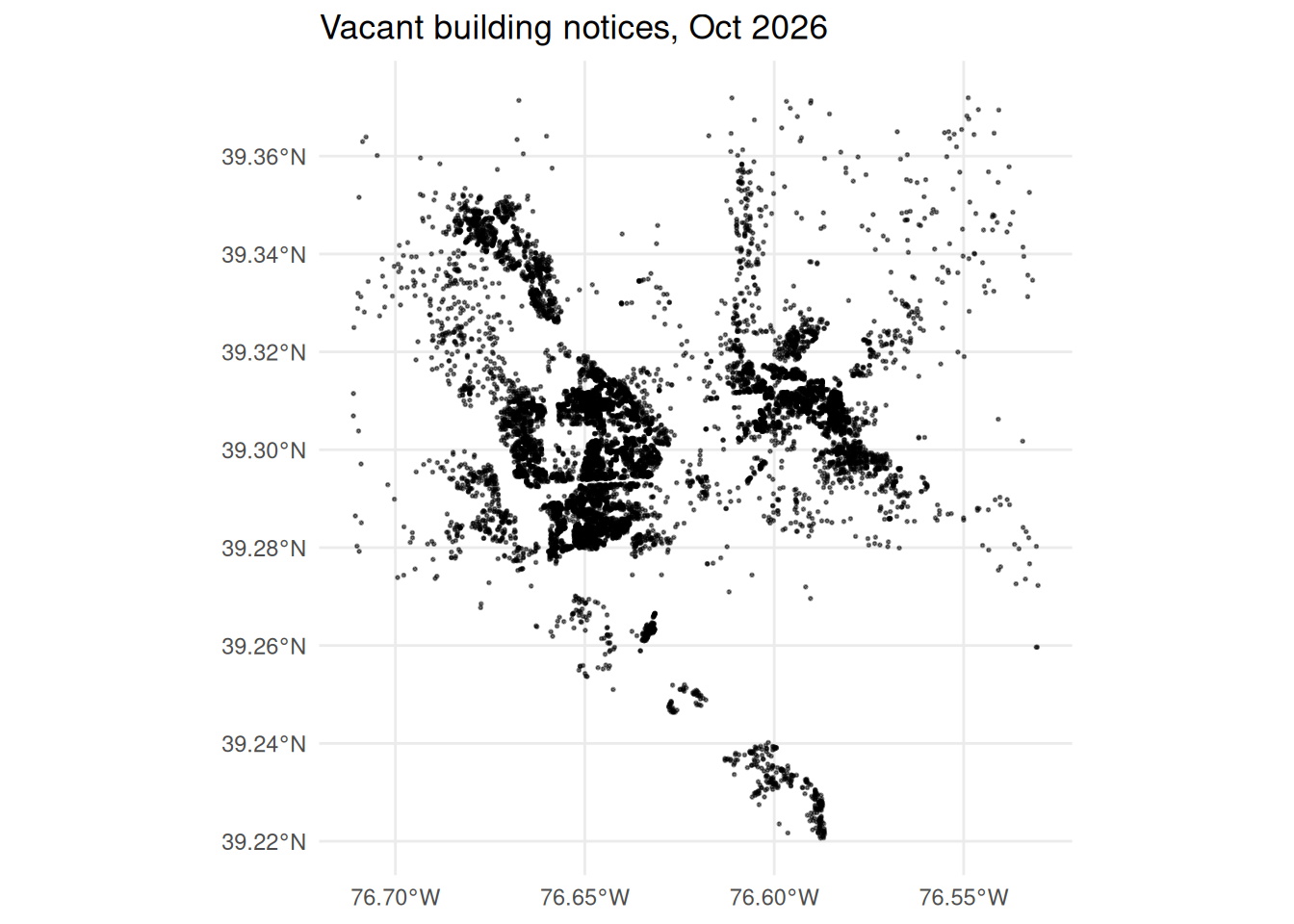
When we have observations that occur at or around specific locations, points can be an easy way to represent them, and you can tack visual encodings onto the points you draw. Color will often work well for this, with the same caveats as nonspatial charts (use good contrast, limit the number of colors you use, use gray for things that need to sink into the background), and with some restrictions that are specific to spatial data (can’t add much jittering to avoid overplotting).
Later we’ll get into some techniques for dealing with overplotting in space, where our story becomes less where individual points are and more where many points tend to cluster.
Code
justviz::vacants_sf |>ggplot() +geom_sf(size =0.3, alpha =0.5) +labs(title ="Vacant building notices, Oct 2026")
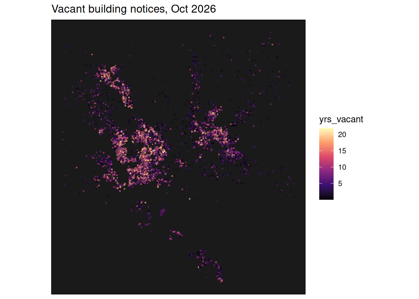
Just from points, knowing a little bit about Baltimore, you can start making out the shapes of neighborhoods from this map of vacancy notices. Using color, you can attach attributes to it.
It can be hard to make lots of small points visible with a sequential palette. The viridis palettes are designed to do this well, especially on a dark background. Other sequential palettes are mostly optimized for filling areas like in choropleths.
Code
# I attached the data I downloaded the data as an attribute on the data framejustviz::vacants_sf |> dplyr::mutate(days_vacant = (as.Date(attr(justviz::vacants_sf, "last_updated")) - date_notice) |>as.numeric() ) |> dplyr::mutate(yrs_vacant = days_vacant /365) |>ggplot(aes(color = yrs_vacant)) +geom_sf(size =0.3, alpha =0.5) +labs(title ="Vacant building notices, Oct 2026") +scale_color_viridis_c(option ="A") +coord_sf(ndiscr =0) +theme(panel.background =element_rect(fill ="gray10"))
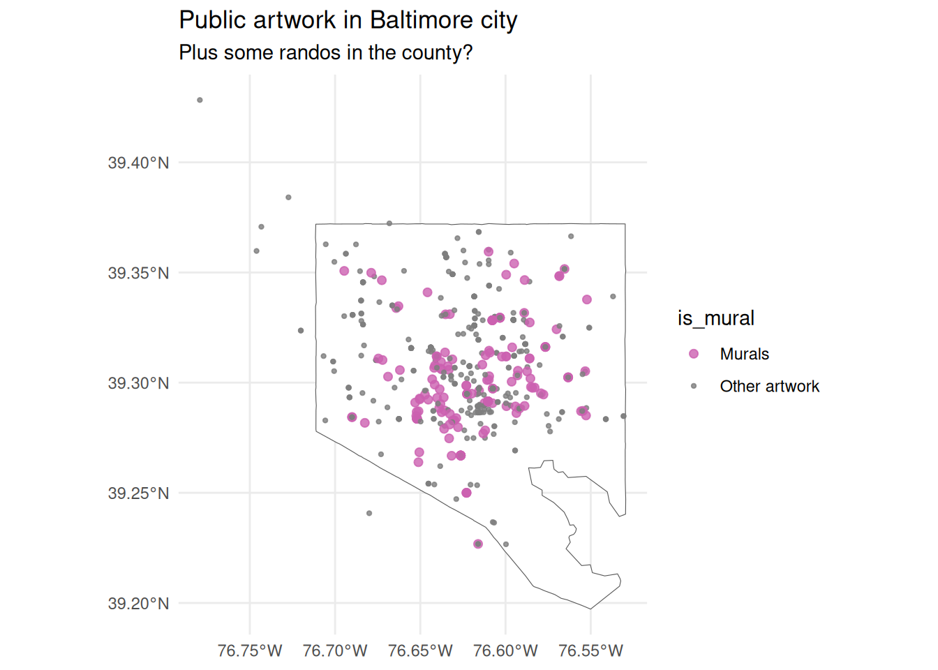
This could also be categorical: here we can use both color and size to highlight murals in the city and let other public artwork sink into the background.
Code
justviz::art_sf |># logical value: does medium contain word "mural" dplyr::mutate(is_mural =ifelse(grepl("mural", medium), "Murals", "Other artwork") ) |>ggplot() +geom_sf(data = counties_sf |> dplyr::filter(county =="Baltimore city"),fill ="white" ) +geom_sf(aes(color = is_mural, size = is_mural), alpha =0.8) +scale_color_manual(values =c("Murals"= qual_pal[5], "Other artwork"="gray50") ) +scale_size_manual(values =c("Murals"=1.8, "Other artwork"=0.8)) +labs(title ="Public artwork in Baltimore city",subtitle ="Plus some randos in the county?" )