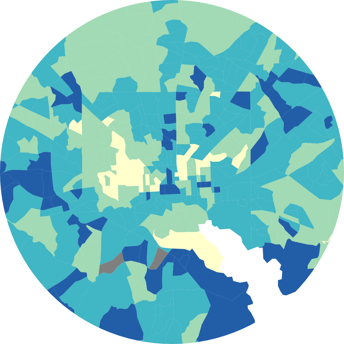
The Census Bureau updates the boundaries of its geographies, such as tracts, after every decennial census. To convert values based on one year's geographies to another year's geographies, you need what's called a crosswalk, or a table of weights to use for averaging values. Unfortunately, many results of the 2020 census were delayed, so some datasets are still put out with 2010 geographies, while others have updated to 2020. The CDC Places data still uses 2010 boundaries, so if you want to merge data from cdc to data from any of the other tract-level datasets, you'll need to use this crosswalk. See the example below.
Format
A data frame with 2052 rows and 3 variables:
- tract20
Character. Tract GEOID based on 2020 geographies.
- tract10
Character. Tract GEOID based on 2010 geographies.
- weight
Numeric. Weight to use in converting values based on 2010 geographies into ones based on 2020 geographies. Use this as the weight for weighted mean calculations.
Examples
head(xwalk_tract_10_to_20)
#> # A tibble: 6 × 3
#>   tract20     tract10      weight
#>   <chr>       <chr>         <dbl>
#> 1 24001000100 24001000100 1
#> 2 24001000200 24001000200 1
#> 3 24001000500 24001000400 0.00493
#> 4 24001000500 24001000500 0.995
#> 5 24001000600 24001000200 0.00903
#> 6 24001000600 24001000600 0.991

# Here's an example walkthrough of how you would prepare the CDC data to join
# it with another dataset---I'll use the EJSCREEN data. I'm filtering each of
# these for the indicators I'm interested in, which are asthma from CDC and
# traffic from EJSCREEN.

library(dplyr)
#>
#> Attaching package: ‘dplyr’
#> The following objects are masked from ‘package:stats’:
#>
#>     filter, lag
#> The following objects are masked from ‘package:base’:
#>
#>     intersect, setdiff, setequal, union

# filter cdc data for just asthma
asthma10 <- cdc |>
  filter(indicator == "Current asthma", level == "tract") |>
  select(tract10 = location, asthma = value, pop)

# calculate values based on 2020 geographies:
# - average asthma rate is calculated as a weighted mean of rates
# - average adult population is calculated as a weighted sum of counts
# (I'm not actually using adult pop for anything, just here as an example of weighting counts)
asthma20 <- asthma10 |>
  inner_join(xwalk_tract_10_to_20, by = "tract10") |>
  group_by(tract20) |>
  summarise(asthma = weighted.mean(asthma, weight),
            adult_pop = sum(pop * weight))

# filter ejscreen for just traffic, rename value column accordingly
traffic <- ejscreen |>
  filter(indicator == "traffic") |>
  select(tract20 = tract, traffic_value_ptile = value_ptile)

# join both data frames now that they have geographies in common
traffic |>
  inner_join(asthma20, by = "tract20")
#> # A tibble: 1,460 × 4
#>    tract20     traffic_value_ptile asthma adult_pop
#>    <chr>                     <int>  <dbl>     <dbl>
#>  1 24001000100                   9  10.4      3718
#>  2 24001000200                   9   9.2      4564
#>  3 24001000500                  83  11.5      2735.
#>  4 24001000600                  45  10.4      2979.
#>  5 24001000700                  47  11.6      3387
#>  6 24001000800                  65  11.9      2213
#>  7 24001001000                  74  11.1      2551.
#>  8 24001001100                  76  10.9      1511.
#>  9 24001001200                  60   9.69     3191.
#> 10 24001001300                  27   9.33     5128.
#> # ℹ 1,450 more rows
